VISUALISATIONS OF ALGEBRAIC PROCESSES AND STRUCTURES

ALGEBRAIC FACTORISATIONS

In general, the story of algebraic factorisation is the story of algebraic expansions reversed. It is reading the distributive law equation from right to left. In the simplest terms, we are to convert an algebraic sum (and/or difference) of groups of unlike terms into a product of factors (containing the greatest number of equal elements in each group). Even the materials used up to now to visualise algebraic expansions can have a twofold purpose, because algebraic rulers (on the left and on the top of geometric representations) help see the factorised forms. However, students in my care convinced me that learners need different semantical explanations of each step to properly and completely factorise any algebraic expression. If I really wanted to maximise the effects of geometric visualisations, I had to not only modify existing visualisations of algebraic expansions but also to create new sets of materials adjusted to reading algebraic equations in the opposite direction. The visualisation of algebraic factorisations opens another window in investigating this matter. Sometimes only when we see things in a mirror we do become aware of the existence of real differences when explaining and elaborating algebraic factorisations successfully.

ONE STAGE FACTORISATIONS

(Algebraic Visualisations 5a)

An introduction into algebraic factorisations can be done using numerical illustrations, to show how and why we do algebraic factorisations. For example:

6 + 8 = 2 × 3 + 2 × 4 = 2 × (3 + 4) = 2 × 7   (adding three and four groups of two);

21 + 6 + 15 = 3 × 7 + 3 × 2 + 3 × 5 = 3 × (7 + 2 + 5) = 3 × 14   (adding seven, two and five groups of three);

16 – 20 + 12 = 4 × 4 – 4 × 5 + 4 × 3 = 4 × (4 – 5 + 3) = 4 × (7 – 5)   (subtracting five groups of four from the sum of four and three groups of four);

Factorisation is another elegant, indispensable tool to be added into our mathematical tool box when doing numerical and/or algebraic operations. Knowing the times timetables is indispensable when doing factorisations because recognising the greatest common factor(s) present in all the terms is essential for doing factorisations successfully.

There are several reasons why we learn to factorise. The addition and subtraction of fractions, their simplification before multiplication, and the division of fractions can be done successfully (without the use of technological devices), only after we have factorised the original numerical or algebraic expression.

If students are taught that each mathematical equation can be read not only from left to right, but from right to left as well, then they already have an idea of how to reverse the already known process of expansion. After explaining that the greatest common factor is placed in front of brackets and that the brackets contain the numbers and/or letters needed to make up the original expression, the process of factorisation should not be a big problem. Geometric visualisations of the process of factorisation help students to fully comprehend this process.

This set of algebraic visualisations consists of the ten most common situations, each having an incrementally more complex starting point in one stage factorisation of algebraic binomials, non-quadratic trinomials and incomplete quadratic trinomials. Some algebraic subtractions are explained in two different ways: as an addition of negative terms and as a subtraction of positive terms. Some students relate better to one way of explanation, some to another; the majority should see their equivalence, if not at once, then after a while. The use of colours helps comprehend this process.

• 5a1 Simple binomial factorisations of the following algebraic forms:
  • n a + n b   and   n a – n b,   [n = 2, 3, 4, 5];
• 5a2 Simple trinomial factorisations of the following algebraic forms:
  • n p + n q + n r   and   n p – n q + n r,   [n = 2, 3, 4];
• 5a3 Simple binomial factorisations of the form:
  • n p + 2 n q,   [n = 2, 3, 4];
• 5a4 Simple binomial factorisations of the form:
  • n a – 3 n b,   [n = 2, 3, 4];
• 5a5 Simple trinomial factorisations of the form:
  • n a + 2 n b + 3 n c,   [n = 2, 3, 4];
• 5a6 Simple trinomial factorisations of the form:
  • 2 n a – n b – 3 n c,   [n = 2, 3, 4];
• 5a7 Simple trinomial factorisations of the form:
  • 2 n a + n a x + 3 n a y,   [n = 2, 3, 4, 5, 6];
• 5a8 Simple trinomial factorisations of the form:
  • 3 n x + n x y – 2 n x z,   [n = 2, 3, 4, 5, 6];
• 5a9 Incomplete quadratic trinomials' factorisations of the form:
  • n x² + 3 n x,   [n = 1, 2, 3];
• 5a10 Incomplete quadratic trinomials' factorisations of the form:
  • 2 n x² – 3 n x,   [n = 1, 2, 3];

TWO-STAGE FACTORISATIONS

(Algebraic Visualisations 5b)

Two-stage factorisations represent a process of grouping unlike terms which contain the same factor(s), their local (first stage) and then their global (second stage) factorisation. This set of Algebraic Visualisations incorporates the typical examples of two-stage factorisations which can be found in any learning environment:

a c + a d + b c + b d;   a c – a d + b c – b d;

- a c + a d – b c + b d;   a c + a d – b c – b d;

a c – a d – b c + b d;   - a c + a d + b c – b d;

- a c – a d + b c + b d;   - a c – a d – b c – b d.

In relation to the nature of grouping we can choose one of the two modes: sequential grouping of terms (1st & 2nd and 3rd & 4th) or alternative grouping of terms (1st & 3rd and 2nd & 4th). As a result, we obtain two seemingly different, but in essence two equivalent outcomes, because they represent an example of the commutative law in multiplication which is present when we do this type of algebraic factorisation in two different ways.

When negative terms are present, it is possible to factorise a four term polynomial only when there is an even number of negative terms. When there is an odd number of negative terms it is not possible to factorise such a four term polynomial.

A frequent question posed by students is when to put a negative term in front of brackets. The typical answer is when you have at least an equal number of positive and negative terms. But it does not have to be only then. The mirror images represent situations in which you put an opposite sign in front of brackets, practically in any situation when factorisation is possible. As a result, you obtain algebraically equivalent situations. It is worthwhile spending some time with students to show them such algebraic realities.

FACTORISATIONS OF QUADRATICS WITH RATIONAL COEFFICIENTS AND REAL FACTORS

(Algebraic Visualisations 5c)

If we want to properly factorise any quadratic trinomial of the form   x² + b x + c   (with a discriminant   b² – 4 a c ≥ 0),   the middle term   b x   must always be split into a sum of   p x + q x,   where   p q = c   and   p + q = b.

There is a systematic investigation of the factors of the constant term   c   at the right corner on each slide and the proper “bingo” combination   (p + q = b)   is highlighted. Only after splitting the middle term into two parts in this way a two-stage factorisation can be performed. The corresponding squares and rectangles (the geometric tools for visualisation) completely illustrate the whole process.

Each situation can be explained using either a general or a summarised mode. The general mode gives images of all the constitutive elements in each situation, while the summarised mode gives an algebraically simplified version. Students can see that any chosen sequence of visualisations represents a fragment of a much greater continuum.

The examples in set 5c1 elaborate the process of factorisation of quadratics of the form   x² ± b x ± c.   When a constant term has zero value   (c = 0)   the quadratic trinomial is being reduced into a quadratic binomial of the form   x² ± b x   and one of the factors is being reduced to a single   x   value   (x ± 0).

The examples in set 5c2 separately elaborate the process of factorisation of quadratics obtained when the   b x   term has zero value (does not exist) and term   c   has a negative value. When this happen, a quadratic trinomial is being reduced into a quadratic binomial of the form   x² – c.   The examples of this type fit into a group called “difference of two squares”. This becomes understandable when we learn that any number   c   represents a squared value of its root. However, the great majority of school examples at this level deal with a   c   value representing a squared value of natural numbers   (c = n²).

The examples in set 5c3 contain quadratics   x² ± b x + c   which can be factorised either as a squared sum or as a squared difference   x² ± 2 x y + y²,   where   2 y = b   and   y² = c.

For me, the greatest accomplishment is achieved when students follow this way of presentation because they are not only able to do algebraic factorisations, but they can explain what they do, how they do it and why they do it that way.

Based on the ideas which encompass rational numbers, I took a step further and incorporated irrational numbers to complement the existing explanations into a bigger mathematical picture when factorising quadratics.

A challenging extension which naturally belongs to the factorisation of this family of quadratic functions, is given in set 5c4. The students are ready for this eye-opening learning experience when they operate at Curriculum Level 7, after they have learned about surds (irrational roots of rational numbers), discriminant   b² – 4 a c,   squaring trinomials and completing the square technique. This is a real example of thinking outside the square in order to factorise any quadratic function with a discriminant    b² – 4 a c ≥ 0.

I have used quadratics   x² ± 2 x – c   although, once the principles explained here are learned, one can take any quadratic of this type and factorise it!

The algebraic situations used in set 5c1 explain how to factorise a quadratic trinomial (when either only the constant term   c   has a negative value or both the   b x   term and the constant term   c   are negative) and could be used for the polynomials factorisation:

y = x² + 2 x – 3   into   y = (x + 3) (x – 1),

y = x² + 2 x – 8   into   y = (x + 4) (x – 2)   etc,   or

y = x² – 2 x – 3   into   y = (x – 3) (x + 1),

y = x² – 2 x – 8   into   y = (x – 4) (x + 2)   etc,

but such a method of factorisation is ineffective when the constant   c   has a size of   c = 1, 2, 4, 5, 6, 7, 9, 10, 11, 12, 13, 14, …   This approach to factorising quadratic trinomials (implemented in set 5c4) is the only way to factorise quadratics   x² + 2 x – c   and   x² – 2 x – c,   which includes cases when   c = 3, c = 8, c = 15, … c = (n² – 1),   n > 1,   and therefore represents a completely new learning experience which is rather difficult to understand without geometric visualisations when learning this kind of algebra. This approach is based on two principles applied one after another: completing the square and the difference of two squares. Anyone who sees this representation will acknowledge that one picture means more than a thousand words!

APPLICATIONS OF RATIONAL QUADRATIC FACTORISATIONS AND EXPANSIONS

(Algebraic Visualisations 5d)

The applications of rational quadratic factorisations and expansions further clarify the purpose of why we do algebraic expansions and factorisations. The known reason is to be able to solve quadratic (and some higher degree) equations without completing the square technique or without using the quadratic formula. Another reason (not mentioned in school textbooks) is to understand the meaning of algebraic equivalence of quadratic functions. This set contains examples made to illustrate algebraic equivalents, to explain how to obtain them and to prove equivalence of the three different forms indirectly (through identical graphical representations) and directly (using algebraic proofs). In essence, it is a set of works illustrating the principle of a quadratic circle and ways how to convert from one form to another.

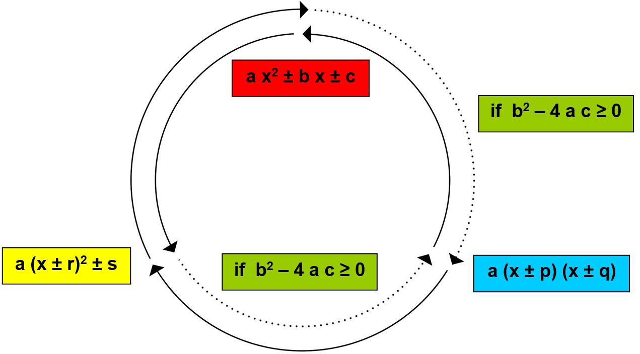
When identifying rules from quadratic patterns we obtain quadratic functions in their expanded form. Any expanded quadratic function   y = a x² ± b x ± c   can always be converted into its vertex form   y = a (x ± r)² ± s   through a process of completing the square (bold inner arc on the quadratic circle diagram in the anticlockwise direction), but it can be converted into its factorised form with use of real factors   y = a (x ± p) (x ± q)   only if the discriminant   b² – 4 a c ≥ 0,   hence this process is represented as a dotted arc. The starting and final point (representing a quadratic function in its expanded form) can be reached again when going along a bold inner arc, because every factorised function can always be converted into its expanded form through a process of algebraic expansion.

When we follow the outer circle in clockwise direction, any expanded quadratic function   y = a x² ± b x ± c   can be converted into its factorised format with use of real factors   y = a (x ± p) (x ± q)   through a process of factorisation only if the discriminant   b² – 4 a c ≥ 0,   hence this process is represented as a dotted arc. Any factorised function   y = a (x ± p) (x ± q)   can always be converted into its vertex format   y = a (x ± r)² ± s   and back into its expanded form   y = a x² ± b x ± c,   hence this pathway is represented with the bold outer arcs on the quadratic circle diagram.

After the the quadratic circle diagram (given in step 1) exemplar 5d1 starts with the graph of a parabola, which in its expanded form has not only all the three terms positive, but they represent a full square as well (step 2). To find intercepts and vertex co-ordinates when a quadratic function is given in this expanded format, we can use postulates of the quadratic formula (step 3), but when it is possible the easiest way is to factorise the expanded quadratic function (step 4). It is easy to find intercepts and vertex co-ordinates of a parabola when a quadratic function is given in this factorised format. Since both factors are identical, they indicate that the   x   intercepts are fused into a single point which represents the vertex as well (step 5). The parabola’s vertex is translated from the origin onto the border between 2nd and 3rd quadrants, in the negative direction of the   x   axis,   r   units left from the origin. It is illustrated in detail in steps 6, 7 and 8. Step 7 illustrates a neat odd number pattern for all parabolas which have a coefficient of   x²   equal to one (a = 1), enabling us to quickly and precisely plot significant points of a parabola when we know the location of its vertex: from the vertex move out 1, up 1, out 1, up 3, out 1, up 5, out 1, up 7, out 1, up 9 and so on. The algebraic proof (step 9) for this situation is trivial but it is given for the purpose of being systematic and coherent with the other exemplars in this set.

All the ten exemplars in set 5d follow the same format outlined in exemplar 5d1, with some inserted extras which were needed to make the conversions between the three different formats fluent.

After the the quadratic circle diagram (given in step 1) exemplar 5d2 starts with the graph of a parabola, which in its expanded form has all the three terms positive, but this time they do not represent a full square. The first extra insert in this exemplar is introduction of the completing the square method to make a conversion from the expanded format into the vertex format of a parabola (step 7). As it can be seen, the method is explained in the three different ways to make this essential process comprehensible for the different type of learners. Students do not need to know all the three ways, but they should be able to align their thinking with at least one of them and assimilate it through some practice. In this example the vertex of a parabola is translated into the 3rd quadrant,   r   units left from the origin,   s   units down.

Another insert is a conversion from the vertex format of a parabola into its factorised form (step 10). This process is explained in two different ways in order to help students completely understand at least one of them, since it is another hurdle which must be overcome during the students’ mathematical cognitive development.

After the the quadratic circle diagram (given in step 1) exemplar 5d3 starts with the graph of a parabola, which in its expanded form has the missing   b x   term   (b x = 0),   the constant term   c   is negative   (c < 0),   and the function has a format of   y = x² – c.   The vertex is translated   c   units under the origin, in the negative direction of the   y   axis, the boundary between the 3rd and 4th quadrants.

After the the quadratic circle diagram (given in step 1) exemplar 5d4 starts with the graph of a parabola, which in its expanded form has only the first quadratic term positive   (a x² > 0)   and the other two terms are negative   (b x < 0   and   c < 0);   its vertex is translated into the 4th quadrant,   r   units right from the origin,   s   units down. Like exemplar 5d2 it represents another full set containing completing the square and a conversion from the vertex format of a parabola into its factorised form.

After the the quadratic circle diagram (given in step 1) exemplar 5d5 starts with the graph of a parabola, which in its expanded form has only the middle   b x   term negative   (b x < 0),   and all the terms together represent a full square. When factorised, both factors are identical, hence they show that   x   intercepts are fused into a single point which represents the vertex as well. The parabola’s vertex is translated onto the boundary between the 4th and 1st quadrants, in the positive direction of the   x   axis,   r   units right from the origin.

Specimens in exemplar 5d5 represent the final example with positive parabolas (having a vertex with a minimum value) which can be equivalently expressed in all three (expanded, factorised and vertex) forms. Positive parabolas whose vertex is above the   x   axis (in the 1st quadrant, on the border between 1st and 2nd quadrants and in the 2nd quadrant) cannot be factorised using rational numbers. They have a negative discriminant   (b² – 4 a c < 0)   and only two (expanded and vertex) forms exist. This problem generates a good moment for giving hints to students that mathematicians developed tools (called complex numbers) for overcoming these problems and making even such quadratic functions factorable. I have developed separate sets to visualise the factorisation of complex quadratics and the factorisation of complex polynomials in the sets named Visual Algebra 3.

In order to finish this circular algebraic journey with the use of rational tools, illustrated by the functions which can be expressed in all the three (expanded, factorised and vertex) forms, we need to consider negative quadratic functions which create graphs of upside-down parabolas (with vertices having a maximum value).

Algebraic visualisations 5d6, 5d7, 5d8, 5d9 and 5d10 contain negative quadratic functions, graphed as upside-down parabolas.

Exemplar 5d6 represents an example of a mirrored mathematical reality in relation to reality illustrated in exemplar 5d5. The vertex form of the parabola is given as   y = - (x – r)²   and for the sake of generating more different learning situations, parabola has been horizontally translated into another position (x_d6 = 4 while x_d5 = 5).

Exemplar 5d7 represents an example of a reflected mathematical reality in relation to reality illustrated in exemplar 5d4. The vertex form of the parabola is given as   y = - (x – r)² + s,   clearly indicating that the vertex is located in the 1st quadrant,   r   units right from the origin,   s   units up.

Exemplar 5d8 represents an example of a mirrored mathematical reality in relation to reality illustrated in exemplar 5d3. The vertex form of the parabola is given as   y = - x² + c,   clearly indicating that the vertex is located   c   units above the origin, on the positive direction of the   y   axis, the boundary between the 1st and 2nd quadrants.

Exemplar 5d9 represents an example of a reflected mathematical reality in relation to reality illustrated in exemplar 5d2. The vertex form of the parabola is given as   y = - (x + r)² + s   clearly indicating that the vertex is located in the 2nd quadrant,   r   units left from the origin,   s   units up.

Finally, exemplar 5d10 represents an example of a mirrored mathematical reality in relation to reality illustrated in exemplar 5d1. The vertex form of the parabola is given as   y = - (x + r)²   clearly indicating that the vertex is located   r   units from the origin, in the negative direction of the   x   axis, the boundary between 2nd and 3rd quadrants.

The ten exemplars in set 5d have been carefully selected so that sets 5d2, 5d4, 5d7 and 5d9 cover increasingly demanding algebraic skills to complete the square and form an equivalent vertex format of parabola of those chosen quadratic functions. Each set contains three different ways showing how I coped with the challenges of explaining this process properly, since I needed to customise the common procedure in order to meet different students’ learning needs. It resulted in having three more or less parallel ways to explain this process of completing the square, but it gave me a real satisfaction when each learner in my care who was able to articulate the problem with his or her understanding finally got their “aha” moment.

The exemplars 5d1, 5d5, 5d6 and 5d10 algebraically represent full squares, so they do not contain the completing the square section. In a similar way sets 5d3 and 5d8 algebraically represent the difference of two squares, so they do not contain completing the square section either.

Sets 5d6, 5d7 and 5d8, with graphical representations located in the first quadrant (including boundaries), contain additional graphical examples of algebraic equivalence when graphing parabolas in factorised form.

All the examples from 5d6 to 5d10 contain unique geometrical illustrations on how to factorise negative quadratic functions and I have not seen these in any mathematical publications so far.

Often, when I was explaining mathematical reality illustrating the squared difference (present in sets 5d5, and 5d6) many students shook their heads in disbelief when they were presented with the fact that (a – b)² = (b – a)². Even after learning algebra for a while and already having relatively good algebraic skills, it was a fascinating learning experience for many students. Again this “algebraic magic” is based on the principle that everything remains the same if multiplied by 1. 1 is the product of (- 1) × (- 1), hence both binomial factors are to be multiplied by (- 1). This transforms the original product of two factors into the product of the two inverted factors, which generates the same, algebraically equivalent, final result:

(a – b)2	=	(a – b) (a – b)
1 (a – b) (a – b)	=	(- 1) (a – b) (- 1) (a – b)
		(- 1) (a – b) (- 1) (a – b)	=	(b – a) (b – a)
				(b – a) (b – a)	=	(b – a)2
(a – b)2	=	(a – b) (a – b)	=	(b – a) (b – a)	=	(b – a)2

With the help of numerical examples this puzzling fact becomes completely logical and can be cemented in students’ heads:

(9 – 5)²   =   4²   =   (5 – 9)²   =   (- 4)²   = 16

(8 – 3)²   =   5²   =   (3 – 8)²   =   (- 5)²   = 25

(7 – 4)²   =   3²   =   (4 – 7)²   =   (- 3)²   =   9

In a similar way we can show that:

(a + b)2	=	(a + b) (a + b)
1 (a + b) (a + b)	=	(- 1) (a + b) (- 1) (a + b)
		(- 1) (a + b) (- 1) (a + b)	=	(- a – b) (- a – b)
				(- a – b) (- a – b)	=	(- a – b)2
(a + b)2	=	(a + b) (a + b)	=	(- a – b) (- a – b)	=	(- a – b)2

Numerical examples help explain this puzzling fact which becomes logical and can be remembered:

(3 + 5)²   =   8²   =   (- 3 – 5)²   =   (- 8)²   =   64

(2 + 7)²   =   9²   =   (- 2 – 7)²   =   (- 9)²   =   81

(1 + 6)²   =   7²   =   (- 1 – 6)²   =   (- 7)²   =   49

Once again, my deep conviction is that meaningful algebra must have daily encounters with numerical and geometrical representations. Otherwise, sooner or later, we start to lose our students on this beautiful journey of their intellectual growth.

TWO-STEP TWO-STAGE FACTORISATIONS WITH A COMMON FACTOR

(Algebraic Visualisations 5e)

In relation to the principles explained in set 5b (two-stage factorisations), exemplars in this set are slightly more sophisticated since all the terms are now multiplied by a constant   n ≥ 1.   In the process of factorising such expressions we need to take a common constant in front of a bracket containing all the terms (the first step) and then, in the second step, we perform their local (the first stage) and global (the second stage) factorisation. As a result we obtain factorised expressions in the form   n (± a ± b) (± c ± d).

To obtain proper representations, when we use this algebraic visualisation, we need to select which terms we want to be positive and which terms we want to be negative when   n = 1   and only after that we can change the size of constant   n.   When negative terms are present, it is possible to factorise a four term polynomial only when there is an even number of negative terms. When there is an odd number of negative terms it is not possible to factorise such a four term polynomial.

Again, the algebraic terms can be ordered either horizontally or vertically, depending on order of grouping of terms containing the same factors.

A frequent question posed by students is when we put a negative term in front of brackets. The typical answer is when you have at least equal number of positive and negative terms. But it does not have to be only then. The mirror images represent situations where you have an opposite sign in front of brackets, practically in any situation when factorisation is possible. As a result, you obtain algebraically equivalent situations. I have found that it is really worthwhile to spend some time with students to show them such algebraic realities.

TWO-STEP TWO-STAGE QUADRATIC FACTORISATIONS WITH A COMMON FACTOR

(Algebraic Visualisations 5f)

The exemplars in this set contain similar algebraic situations (in relation to the exemplars contained in set 5e) with a slight variation caused by the fact that sometimes   c = a   which consequently produces a quadratic situation. Algebraically, when factorised, it means that

n (± a ± b) (± c ± d)   when   c = a   becomes   n (± a ± b) (± a ± d).

To obtain proper representations, when we use this algebraic visualisation, we need to select which terms we want to be positive and which terms we want to be negative when   n = 1   and only then can we change the size of constant   n.   When negative terms are present, it is possible to factorise a four term quadratic polynomial only when there is an even number of negative terms. When there is an odd number of negative terms it is not possible to factorise such a four term polynomial. Again, in this set, the factorised quadratics are ordered either horizontally or vertically. In any situation when factorisation is possible there is a possibility to create mirror images. These represent situations when you deliberately choose an opposite sign in front of the brackets. It is beneficial for our students to see that, as a result, we obtain algebraically equivalent situations.

EXAMPLES OF TWO-STEP TWO-STAGE QUADRATIC FACTORISATIONS WITH A COMMON FACTOR

(Algebraic Visualisations 5g)

The exemplars in set 5g1 illustrate two-step two-stage factorisations of quadratic trinomials having a common factor and expressed in the form:

• 5g1a   n (x² + b x + c),   [n = 1, 2, 3, 4, 5, 6];
• 5g1b   n (x² – b x – c),   [n = 1, 2, 3, 4, 5, 6];
• 5g1c   n (x² + b x – c),   [n = 1, 2, 3, 4, 5, 6];
• 5g1d   n (x² – b x + c),   [n = 1, 2, 3, 4, 5, 6];

The exemplars in set 5g2 contain algebraic visualisations of multiples of difference of two squares   n (x² – y²),   [n = 1, 2, 3, 4, 5, 6];

while the exemplars in set 5g3 contain algebraic visualisations of multiples of squared sums or multiples of squared differences   n (x² ± 2 x y + y²),   [n = 1, 2, 3, 4, 5, 6].

Such quadratics geometrically can be ordered horizontally, vertically or using a combination of those two approaches. If I could have the tools to project these realities onto larger surfaces, then I could have (as already shown in set 5f) only horizontal or only vertical arrangements. Since I did not have such tools I had to create combined groups of identical building blocks. Nevertheless, neither algebra, nor geometry have been compromised and the enclosed examples realistically represent such algebraic situations. The beauty of this set can be found in expressing the same quadratic reality looked at from another perspective.

TWO-STEP TWO-STAGE QUADRATIC FACTORISATIONS WITHOUT A COMMON FACTOR

(Algebraic Visualisations 5h)

It is really interesting to see how many different ways textbooks have been offering for this type of factorisation of quadratics. The evolution of this method culminated with creation of this universal method, being very similar to those already described and used. It can be easily represented geometrically and understood by students.

Any rational quadratic function can be expressed as   y = a x² + b x + c.   If we want to factorise it, the middle   b x   term must always be split into   p x + q x,   where   p q = a c   and   p + q = b.   Only after splitting the middle term into two parts in this way a two-stage factorisation can be performed. In relation to the already known procedure of factorising rational quadratics, there is no change at all. The only difference is that before we had simpler quadratics with   a = 1   which reduced   y = a x² + b x + c   into   y = (1) x² + b x + c   and hence the requirement   p q = a c   was reduced to   p q = (1) c.   This means that the procedure of factorising simpler quadratics is a special case contained within this general one, encompassing all situations. When students see and understand this difference they never have problems with these “difficult” types of quadratic factorisations. The materials in this set realistically visualise and geometrically illustrate the whole process.

The most frequent students’ question is what order we use when ordering   p x   and   q x   terms during the factorisation process. The answer is that it really does not matter. The first four exemplars (5h1 to 5h4) were created to show that there is no difference when we have a different (inverted) order of   p x   and   q x   terms after splitting the middle   b x   term into two parts. The only difference is that (geometrically) one way generates a horizontal grouping of terms and the other produces a vertical grouping of terms. In the end (algebraically) those two ways create two identical factors, which are placed in inverted order. This makes no real difference (the inverted factors represent an algebraic equivalence) since the commutative law can always be implemented in the multiplication of factors. The first four exemplars convincingly illustrate this algebraic reality:

• 5h1   a x² + b x + c   with both horizontal and vertical grouping of terms;
• 5h2   a x² + b x – c   with both horizontal and vertical grouping of terms;
• 5h3   a x² – b x – c   with both horizontal and vertical grouping of terms;
• 5h4   a x² – b x + c   with both horizontal and vertical grouping of terms;

After clarifying this situation, the next set of four exemplars (5h5 to 5h8) is focused at providing a bigger picture about two-step two-stage quadratic factorizations without a common factor.

• 5h5    a x² + b x + c   visualises four basic linked examples;
• 5h6    a x² – b x – c   visualises four basic linked examples;
• 5h7    a x² + b x – c   visualises five basic linked examples;
• 5h8    a x² – b x + c   visualises five basic linked examples;

The next four sets of algebraic visualisations (5h9 to 5h12) were created to show that this method of algebraic factorisation represents a universal method of quadratic factorisation that creates factors which are given in the following forms:

(d x + e) (f x + g),   (d x + e) (f x – g),   (d x – e) (f x + g),   (d x – e) (f x – g).

• 5h9    a x² + b x + c   visualised as four sophisticated linked examples;
• 5h10    a x² + b x – c   visualised as four sophisticated linked examples;
• 5h11    a x² – b x – c   visualised as four sophisticated linked examples;
• 5h12    a x² – b x + c   visualised as four sophisticated linked examples;

Sets 5h13 and 5h14 represent situations which, when factorised, can be expressed as (multiples of) squared sums   n (a x + b)²   and   (multiples of) squared differences   n (a x – b)²,   while set 5h15 represents (multiples of) differences of two squares   n (a x + b) (a x – b)   or   n (a x – b) (a x + b).

• 5h13    a x² + b x + c   visualised as three linked more sophisticated examples;
• 5h14    a x² – b x + c   visualised as three linked more sophisticated examples;
• 5h15    a x² – c   visualised as three linked more sophisticated examples;

The last two exemplars in this set (5h16 and 5h17) were created to show that we still have exceptional cases which cannot be fully encompassed by this “universal” method of quadratic factorisation. Such atypical situations can be encountered when we have incomplete quadratics with   c = 0.   The factorisation requirement   p q = a c   is deformed into   p q = 0,   since   c = 0.   This makes   q = 0,   because   p ≠ 0.   As a consequence we have incomplete quadratics elaborated in 5h16   a x² + b x,   factorised as   (d x + e) (f x + 0) = f x (d x + e),   and incomplete quadratics elaborated in 5h17   a x² – b x,  factorised as   (d x – e) (f x + 0) = f x (d x – e).   Both situations can be understood and identified as “enriched” factorisation of binomials.

THREE-STEP QUADRATIC FACTORISATIONS

(Algebraic Visualisations 6)

The final stage of rational quadratic factorisations finishes with four typical exemplars of three-step quadratic factorisations illustrated and explained in the four sets: 6a, 6b, 6c and 6d. In relation to previous cases we take a common factor in front of brackets, then we break the middle b x term in the already learned process into two segments   p x   and   q x,   and finally we perform local and global factorisations. These concepts represent a final stage for a great majority of our secondary students (before introduction of complex numbers), creating an impressive big view into rational quadratic factorisations.

• 6a    n (a x² + b x + c)   visualised as factorised examples   n (d x + e) (f x + g);
• 6b    n (a x² ± b x – c)   visualised as factorised examples   n (d x – e) (f x + g);
• 6c    n (a x² ± b x – c)   visualised as factorised examples   n (d x + e) (f x – g);
• 6d    n (a x² – b x + c)   visualised as factorised examples   n (d x – e) (f x – g).

Unfortunately, my attempts to create more resources of this type failed, since the constitutive components became too small and, in the end, illegible for A4 formats. However, from my experience I can confidently say that students can perform these types of factorisations without significant difficulties and are able to describe the detailed arrangement and composition of such algebraic structures.

FACTORISATIONS OF POLYNOMIALS and EXTENSION MATERIALS